- Foreword
- 1. Introduction
- 2. Model, Cost Function and Gradient Descent
- 3. Linear Regression
- 4. Logistic Regression
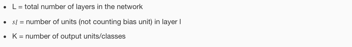
- 5. Neural Network
- 6. Support Vector Machines
- 7. Clustering
- 8. Anomaly Detection
- 9. Tips for Building a Learning System
Foreword
Study notes for Machine Learning Course by Andrew Ng on Coursera.
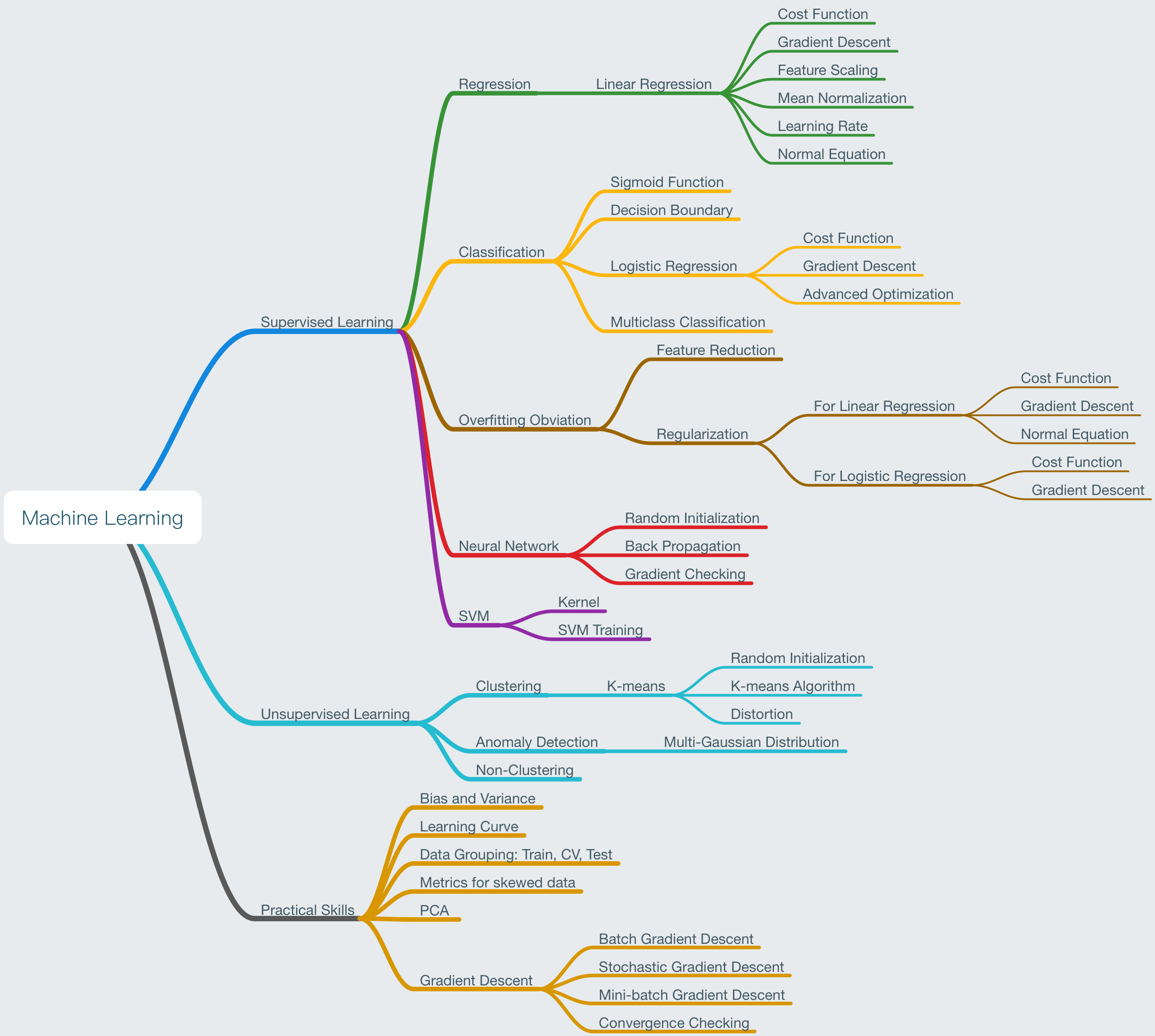
Mind Mapping for this course:
1. Introduction
1.1 Machine Learning Definition
Tom Mitchell provides a more modern definition: “A computer program is said to learn from experience E with respect to some class of tasks T and performance measure P, if its performance at tasks in T, as measured by P, improves with experience E.”
Example: playing checkers.
E = the experience of playing many games of checkers
T = the task of playing checkers.
P = the probability that the program will win the next game.
1.2 Supervised and Unsupervised Learning
In supervised learning, we are given a data set and already know what our correct output should look like, having the idea that there is a relationship between the input and the output.
Supervised learning problems are categorized into “regression” and “classification” problems. In a regression problem, we are trying to predict results within a continuous output, meaning that we are trying to map input variables to some continuous function. In a classification problem, we are instead trying to predict results in a discrete output. In other words, we are trying to map input variables into discrete categories.
Unsupervised learning allows us to approach problems with little or no idea what our results should look like. We can derive structure from data where we don’t necessarily know the effect of the variables.
We can derive this structure by clustering the data based on relationships among the variables in the data.
2. Model, Cost Function and Gradient Descent
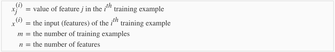
2.1 Model
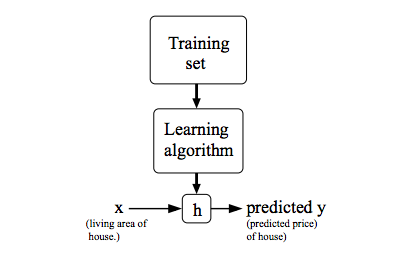
Given a training set, to learn a function h : X → Y so that h(x) is a “good” predictor for the corresponding value of y. For historical reasons, this function h is called a hypothesis.
2.2 Cost Function

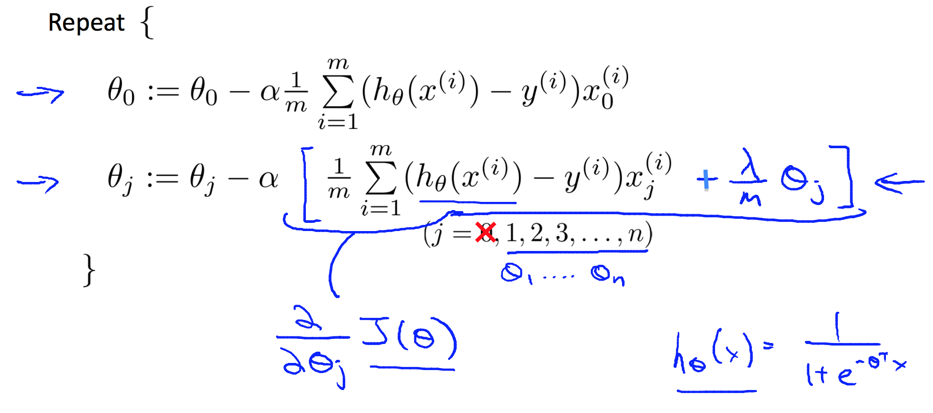
(1/2) is for gradient descent convenience. lambda is called the regularization parameter.
2.3 Gradient Descent
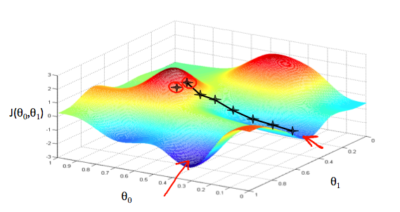
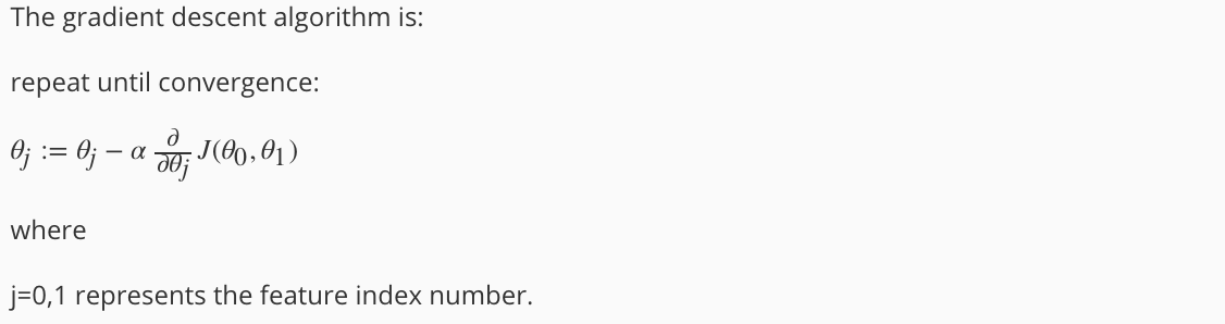
α is called Learning Rate.
3. Linear Regression
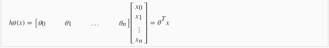
3.1 Model
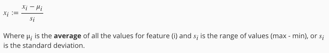
3.2 Feature Scaling and Mean Normalization
% matlab code for feature scaling and mean normalization
mu = mean(X);
sigma = std(X);
for i = 1:size(X,2)
    X_norm(:,i) = (X(:,i)-mu(i))/sigma(i);
end
3.3 Learning Rate
Make a plot with number of iterations on the x-axis. Now plot the cost function, J(θ) over the number of iterations of gradient descent. If J(θ) ever increases, then you probably need to decrease α.
3.4 Cost function and Gradient Descent
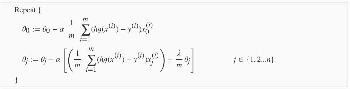
% Cost function and gradient for linear regression
J = sum((X * theta - y).^2)/(2*m) + + lambda/(2 * m) * sum(theta(2:end).^2);

grad = X' * (X * theta - y) / m + [0; lambda * theta(2:end) / m];
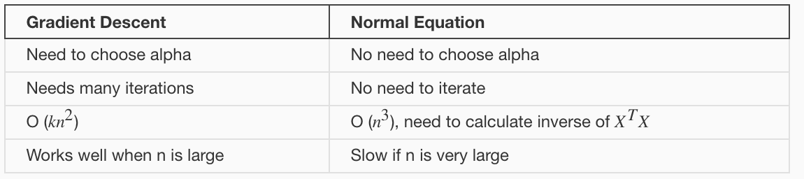
3.5 Normal Equation
A closed-form solution to linear regression is:
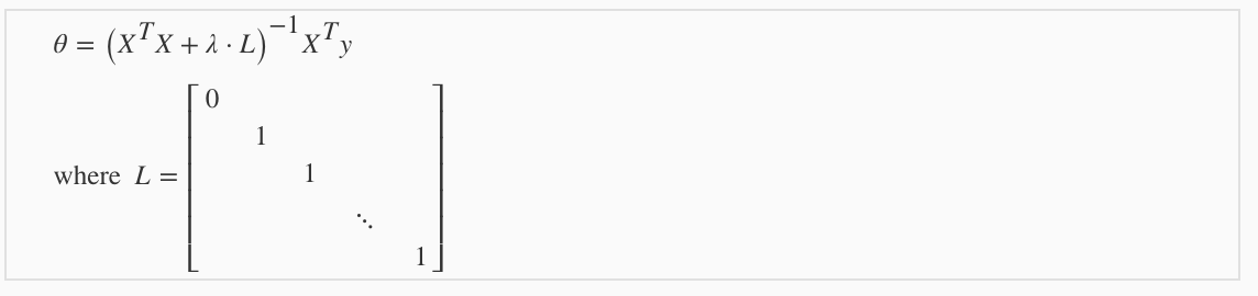
% matlab code for normal equation
theta = pinv(X' * X + lambda * L) * X' * y;
4. Logistic Regression
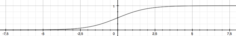
4.1 Model
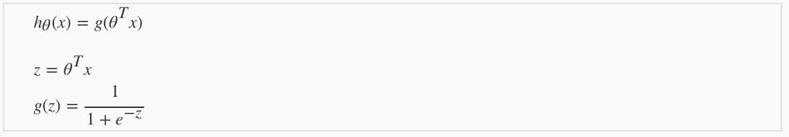
g(z) is called the ‘sigmoild function’ or ‘logistic function’.
4.2 Cost Function and Gradient Descent

% matlab code for cost function and gradient of logistic regression
h = sigmoid(X * theta);
n = length(theta);
J = (-y' * log(h)- (1 - y)' * log(1 - h)) / m + lambda/(2 * m) * sum(theta(2:n).^2);
grad = X' * (h - y) / m + [0; lambda * theta(2:n) / m];
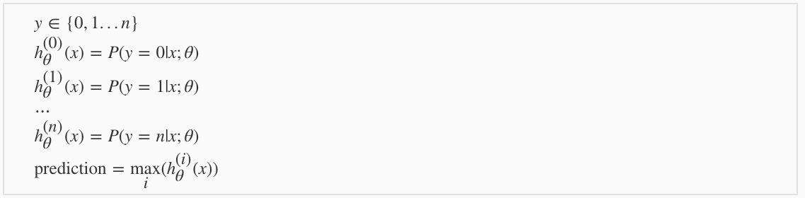
4.3 Multiclass Classification
One-vs-all method:
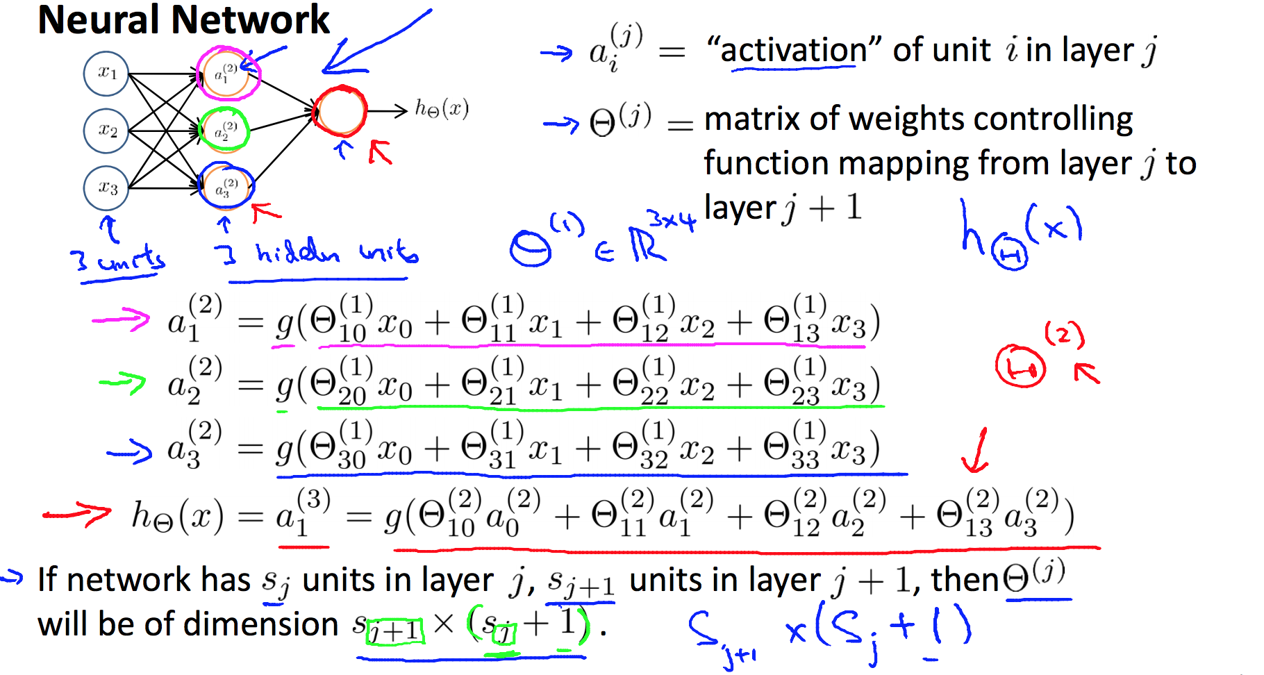
5. Neural Network
5.1 Model
5.2 Cost Function

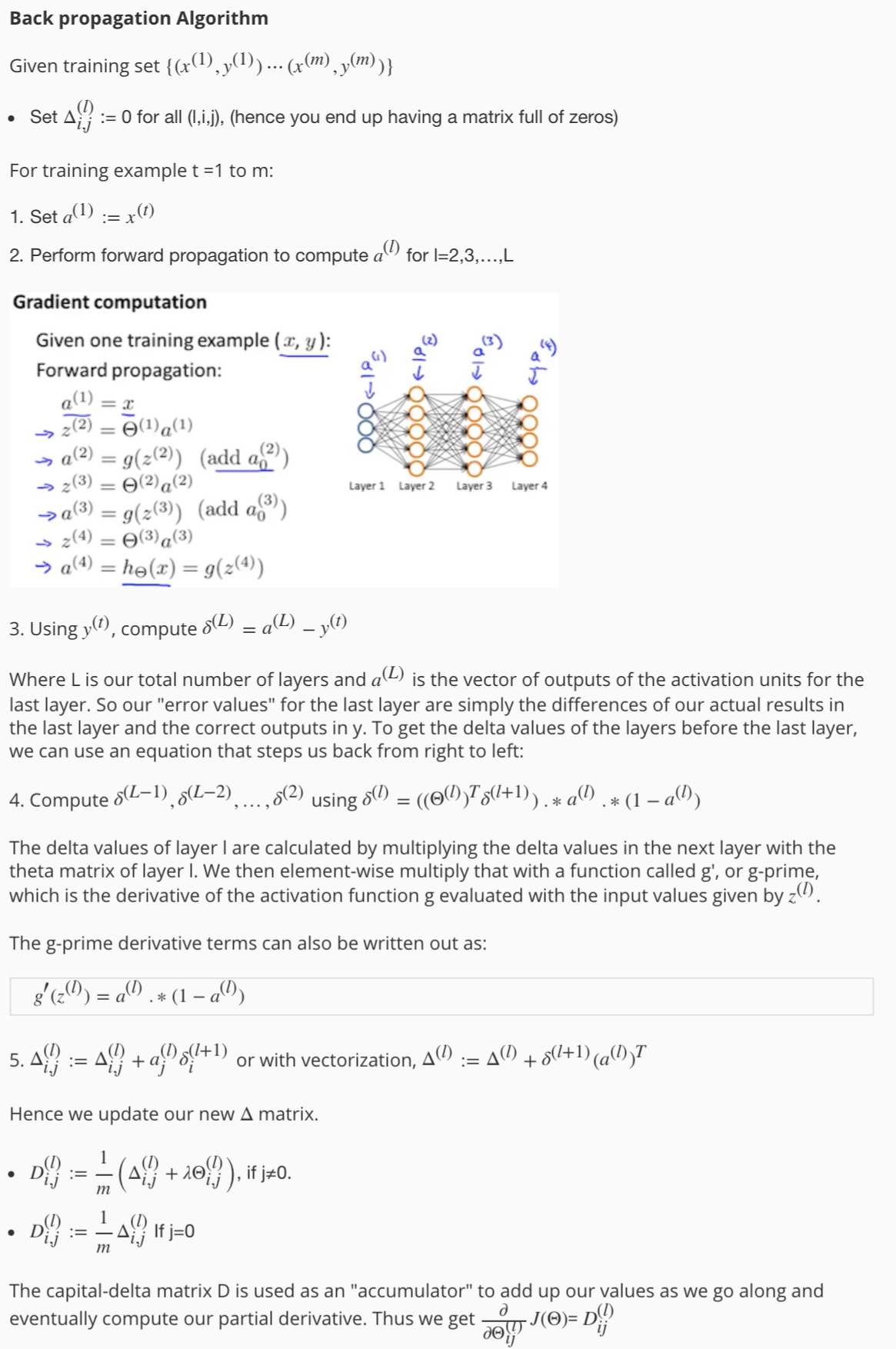
5.3 Back Propagation
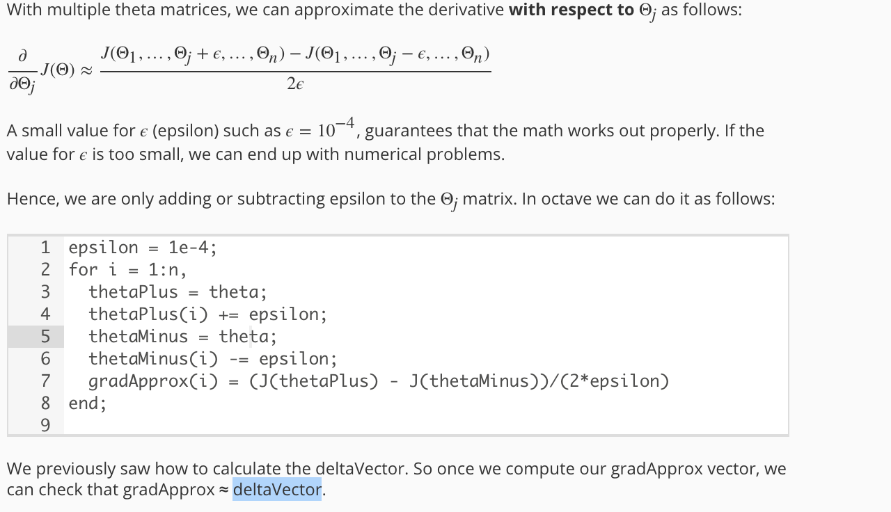
5.4 Gradient Checking
function numgrad = computeNumericalGradient(J, theta)
%COMPUTENUMERICALGRADIENT Computes the gradient using "finite differences"
%and gives us a numerical estimate of the gradient.
%   numgrad = COMPUTENUMERICALGRADIENT(J, theta) computes the numerical
%   gradient of the function J around theta. Calling y = J(theta) should
%   return the function value at theta.

% Notes: The following code implements numerical gradient checking, and
%        returns the numerical gradient.It sets numgrad(i) to (a numerical
%        approximation of) the partial derivative of J with respect to the
%        i-th input argument, evaluated at theta. (i.e., numgrad(i) should
%        be the (approximately) the partial derivative of J with respect
%        to theta(i).)
%

numgrad = zeros(size(theta));
perturb = zeros(size(theta));
e = 1e-4;
for p = 1:numel(theta)
    % Set perturbation vector
    perturb(p) = e;
    loss1 = J(theta - perturb);
    loss2 = J(theta + perturb);
    % Compute Numerical Gradient
    numgrad(p) = (loss2 - loss1) / (2*e);
    perturb(p) = 0;
end

end
function checkNNGradients(lambda)
%CHECKNNGRADIENTS Creates a small neural network to check the
%backpropagation gradients
%   CHECKNNGRADIENTS(lambda) Creates a small neural network to check the
%   backpropagation gradients, it will output the analytical gradients
%   produced by your backprop code and the numerical gradients (computed
%   using computeNumericalGradient). These two gradient computations should
%   result in very similar values.
%

if ~exist('lambda', 'var') || isempty(lambda)
    lambda = 0;
end

input_layer_size = 3;
hidden_layer_size = 5;
num_labels = 3;
m = 5;

% We generate some 'random' test data
Theta1 = debugInitializeWeights(hidden_layer_size, input_layer_size);
Theta2 = debugInitializeWeights(num_labels, hidden_layer_size);
% Reusing debugInitializeWeights to generate X
X  = debugInitializeWeights(m, input_layer_size - 1);
y  = 1 + mod(1:m, num_labels)';

% Unroll parameters
nn_params = [Theta1(:) ; Theta2(:)];

% Short hand for cost function
costFunc = @(p) nnCostFunction(p, input_layer_size, hidden_layer_size, ...
                               num_labels, X, y, lambda);

[cost, grad] = costFunc(nn_params);
numgrad = computeNumericalGradient(costFunc, nn_params);

% Visually examine the two gradient computations.  The two columns
% you get should be very similar.
disp([numgrad grad]);
fprintf(['The above two columns you get should be very similar.\n' ...
         '(Left-Your Numerical Gradient, Right-Analytical Gradient)\n\n']);

% Evaluate the norm of the difference between two solutions.
% If you have a correct implementation, and assuming you used EPSILON = 0.0001
% in computeNumericalGradient.m, then diff below should be less than 1e-9
diff = norm(numgrad-grad)/norm(numgrad+grad);

fprintf(['If your backpropagation implementation is correct, then \n' ...
         'the relative difference will be small (less than 1e-9). \n' ...
         '\nRelative Difference: %g\n'], diff);

end
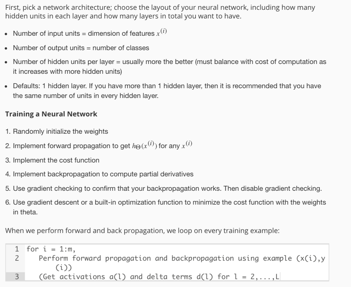
5.5 Neural Network Learning Steps
function [J grad] = nnCostFunction(nn_params, ...
                                   input_layer_size, ...
                                   hidden_layer_size, ...
                                   num_labels, ...
                                   X, y, lambda)
%NNCOSTFUNCTION Implements the neural network cost function for a two layer
%neural network which performs classification
%   [J grad] = NNCOSTFUNCTON(nn_params, hidden_layer_size, num_labels, ...
%   X, y, lambda) computes the cost and gradient of the neural network. The
%   parameters for the neural network are "unrolled" into the vector
%   nn_params and need to be converted back into the weight matrices.
%
%   The returned parameter grad should be a "unrolled" vector of the
%   partial derivatives of the neural network.
%

% Reshape nn_params back into the parameters Theta1 and Theta2, the weight matrices
% for our 2 layer neural network
Theta1 = reshape(nn_params(1:hidden_layer_size * (input_layer_size + 1)), ...
                 hidden_layer_size, (input_layer_size + 1));

Theta2 = reshape(nn_params((1 + (hidden_layer_size * (input_layer_size + 1))):end), ...
                 num_labels, (hidden_layer_size + 1));

% Setup some useful variables
m = size(X, 1);

% You need to return the following variables correctly
J = 0;
Theta1_grad = zeros(size(Theta1));
Theta2_grad = zeros(size(Theta2));

% Instructions: You should complete the code by working through the
%               following parts.
%
% Part 1: Feedforward the neural network and return the cost in the
%         variable J. After implementing Part 1, you can verify that your
%         cost function computation is correct by verifying the cost
%         computed in ex4.m
%
% Part 2: Implement the backpropagation algorithm to compute the gradients
%         Theta1_grad and Theta2_grad. You should return the partial derivatives of
%         the cost function with respect to Theta1 and Theta2 in Theta1_grad and
%         Theta2_grad, respectively. After implementing Part 2, you can check
%         that your implementation is correct by running checkNNGradients
%
%         Note: The vector y passed into the function is a vector of labels
%               containing values from 1..K. You need to map this vector into a
%               binary vector of 1's and 0's to be used with the neural network
%               cost function.
%
%         Hint: We recommend implementing backpropagation using a for-loop
%               over the training examples if you are implementing it for the
%               first time.
%
% Part 3: Implement regularization with the cost function and gradients.
%
%         Hint: You can implement this around the code for
%               backpropagation. That is, you can compute the gradients for
%               the regularization separately and then add them to Theta1_grad
%               and Theta2_grad from Part 2.
%

yVec = zeros(m, num_labels);
for i = 1:length(y)
    yVec(i,y(i)) = 1;
end

%% =================== feedforward ===========
% 5000*401
X = [ones(m,1) X];
% 5000*26
A2 = [ones(m,1) sigmoid(X * Theta1')];
% 5000*10
A3 = sigmoid(A2 * Theta2');
J = sum(-dot(yVec', log(A3)') - dot((1 - yVec)', log(1 - A3)')) / m;

% Regularization
th1 = Theta1(:,2:end).^2;
th2 = Theta2(:,2:end).^2;
J = J + lambda / (2 * m) * (sum(th1(:)) +sum(th2(:)));


%% ================== backpropagation ============

for t = 1:m
    % step1 feedforward to calculate a1 z2 a2 z3 a3
    % 401*1
    a1 = X(t,:)';
    % 26*1
    z2 = Theta1 * a1;
    a2 = [1; sigmoid(z2)];
    %10*1
    z3 = Theta2 * a2;
    a3 = sigmoid(z3);

    % step2 calculate detal3 and delta2
    % 10*1
    delta3 = a3 - yVec(t,:)';
    % 26*1
    delta2 = Theta2' * delta3 .* [0; sigmoidGradient(z2)];

    % step3 accumulate the gradient
    Theta2_grad = Theta2_grad + delta3 * a2';
    Theta1_grad = Theta1_grad + delta2(2:end) * a1';
end

Theta2_grad = Theta2_grad / m + lambda * [zeros(num_labels, 1) Theta2(:, 2:end)] / m;
Theta1_grad = Theta1_grad / m + lambda * [zeros(hidden_layer_size, 1) Theta1(:, 2:end)] / m;


%% -------------------------------------------------------------

% =========================================================================

% Unroll gradients
grad = [Theta1_grad(:) ; Theta2_grad(:)];


end
6. Support Vector Machines
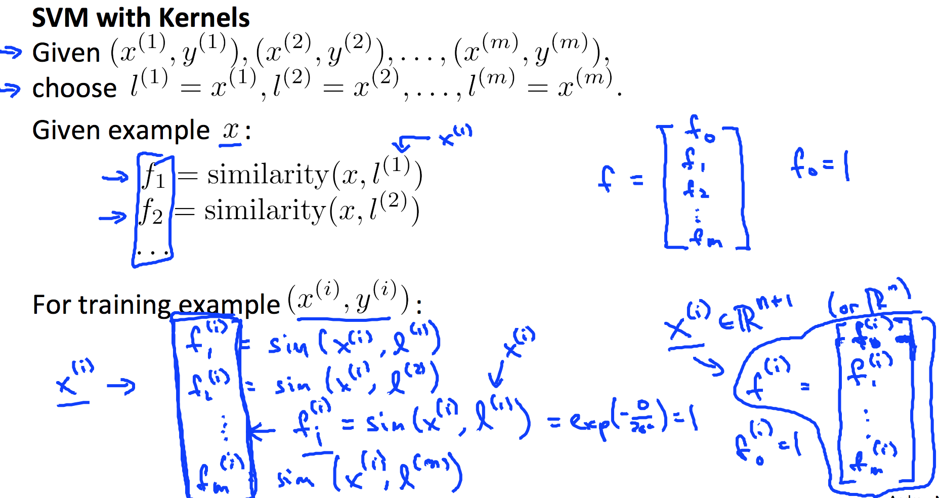
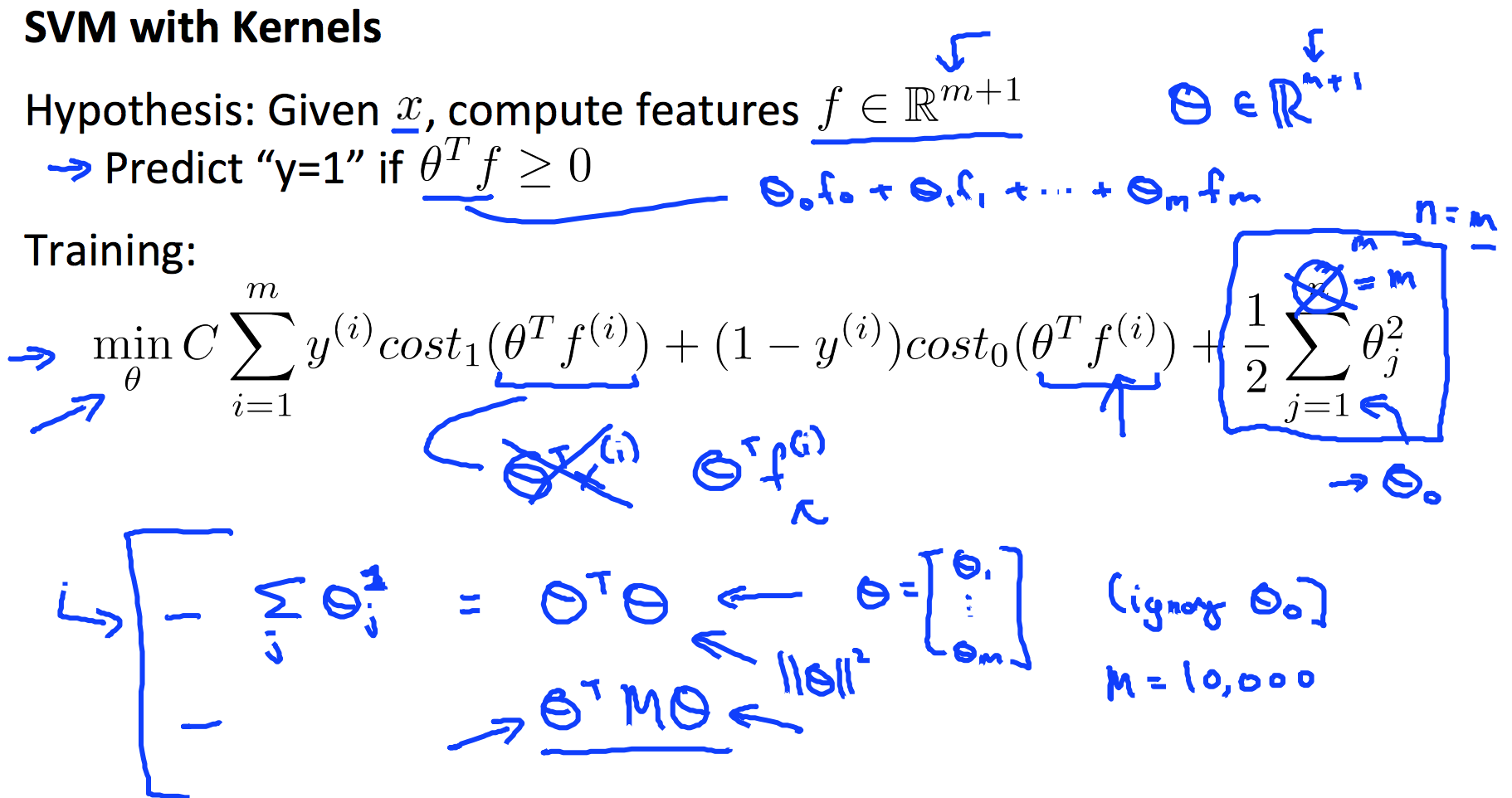
6.1 Kernel

Do perform feature scaling before using the Gaussian Kernel.
Other kernels: Polynomial kernel, String kernel, Chi-square kernel, Histogram intersection kernel.
function sim = linearKernel(x1, x2)
%LINEARKERNEL returns a linear kernel between x1 and x2
%   sim = linearKernel(x1, x2) returns a linear kernel between x1 and x2
%   and returns the value in sim

% Ensure that x1 and x2 are column vectors
x1 = x1(:); x2 = x2(:);

% Compute the kernel
sim = x1' * x2;  % dot product

end
function sim = gaussianKernel(x1, x2, sigma)
%RBFKERNEL returns a radial basis function kernel between x1 and x2
%   sim = gaussianKernel(x1, x2) returns a gaussian kernel between x1 and x2
%   and returns the value in sim

% Ensure that x1 and x2 are column vectors
x1 = x1(:); x2 = x2(:);

% You need to return the following variables correctly.
sim = 0;

% Instructions: Fill in this function to return the similarity between x1
%               and x2 computed using a Gaussian kernel with bandwidth
%               sigma
%
%
sim = exp(- sum((x1 - x2) .^ 2) /  (sigma ^ 2 * 2));

end
6.2 SVM Train and Prediction
Use toolbox like LIBSVM to do svm training. Steps below is just an overview.
- Choose every x as l;
- Choose kernel function;
- Feature scaling;
- Choose best C (and sigma, if you use Gaussian Kernel);
- Use libsvm or other libraries to train svm model;
- Make prediction and test on cross validation data.
function pred = svmPredict(model, X)
%SVMPREDICT returns a vector of predictions using a trained SVM model
%(svmTrain).
%   pred = SVMPREDICT(model, X) returns a vector of predictions using a
%   trained SVM model (svmTrain). X is a mxn matrix where there each
%   example is a row. model is a svm model returned from svmTrain.
%   predictions pred is a m x 1 column of predictions of {0, 1} values.
%

% Check if we are getting a column vector, if so, then assume that we only
% need to do prediction for a single example
if (size(X, 2) == 1)
    % Examples should be in rows
    X = X';
end

% Dataset
m = size(X, 1);
p = zeros(m, 1);
pred = zeros(m, 1);

if strcmp(func2str(model.kernelFunction), 'linearKernel')
    % We can use the weights and bias directly if working with the
    % linear kernel
    p = X * model.w + model.b;
elseif strfind(func2str(model.kernelFunction), 'gaussianKernel')
    % Vectorized RBF Kernel
    % This is equivalent to computing the kernel on every pair of examples
    X1 = sum(X.^2, 2);
    X2 = sum(model.X.^2, 2)';
    K = bsxfun(@plus, X1, bsxfun(@plus, X2, - 2 * X * model.X'));
    K = model.kernelFunction(1, 0) .^ K;
    K = bsxfun(@times, model.y', K);
    K = bsxfun(@times, model.alphas', K);
    p = sum(K, 2);
else
    % Other Non-linear kernel
    for i = 1:m
        prediction = 0;
        for j = 1:size(model.X, 1)
            prediction = prediction + ...
                model.alphas(j) * model.y(j) * ...
                model.kernelFunction(X(i,:)', model.X(j,:)');
        end
        p(i) = prediction + model.b;
    end
end

% Convert predictions into 0 / 1
pred(p >= 0) =  1;
pred(p <  0) =  0;

end
6.3 Logistic Regrssion vs. SVM
n = number of feature, m = number of training examples.
If n is large (relative to m): Use logistic regression, or SVM without a kernel (linear kernel).
If n is small, m is intermediate: Use SVM with Gaussian kernel.
If n is small, m is large: Create/add more features, then use logistic regression or SVM without a kernel.
Neural network likely to work well for most of these settings, but may be slower to train.
7. Clustering
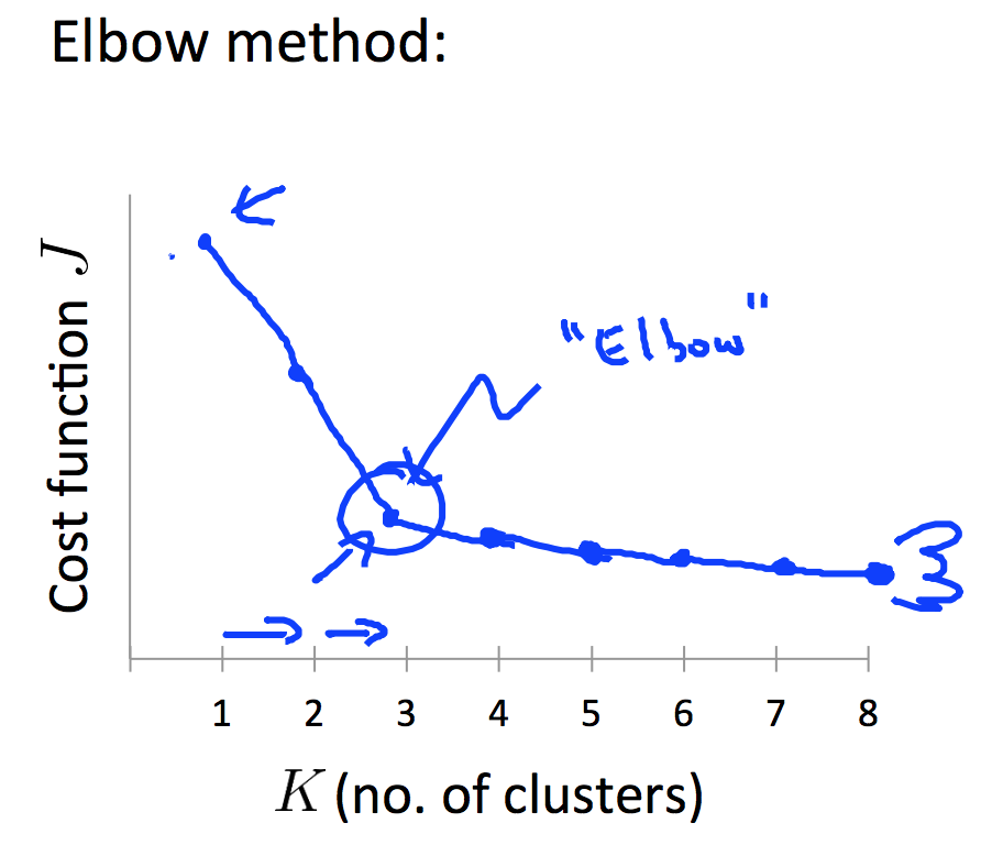
7.1 K-means
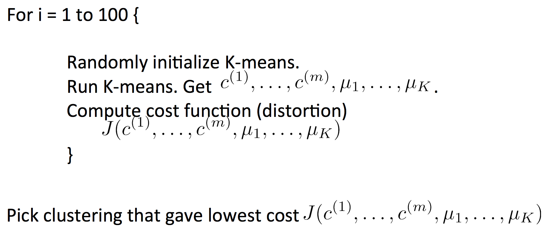
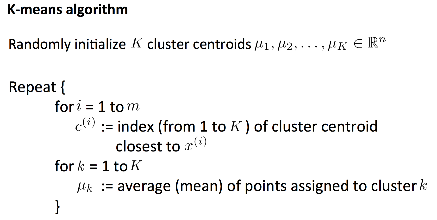
You can use the Elbow Method to choose K.
8. Anomaly Detection
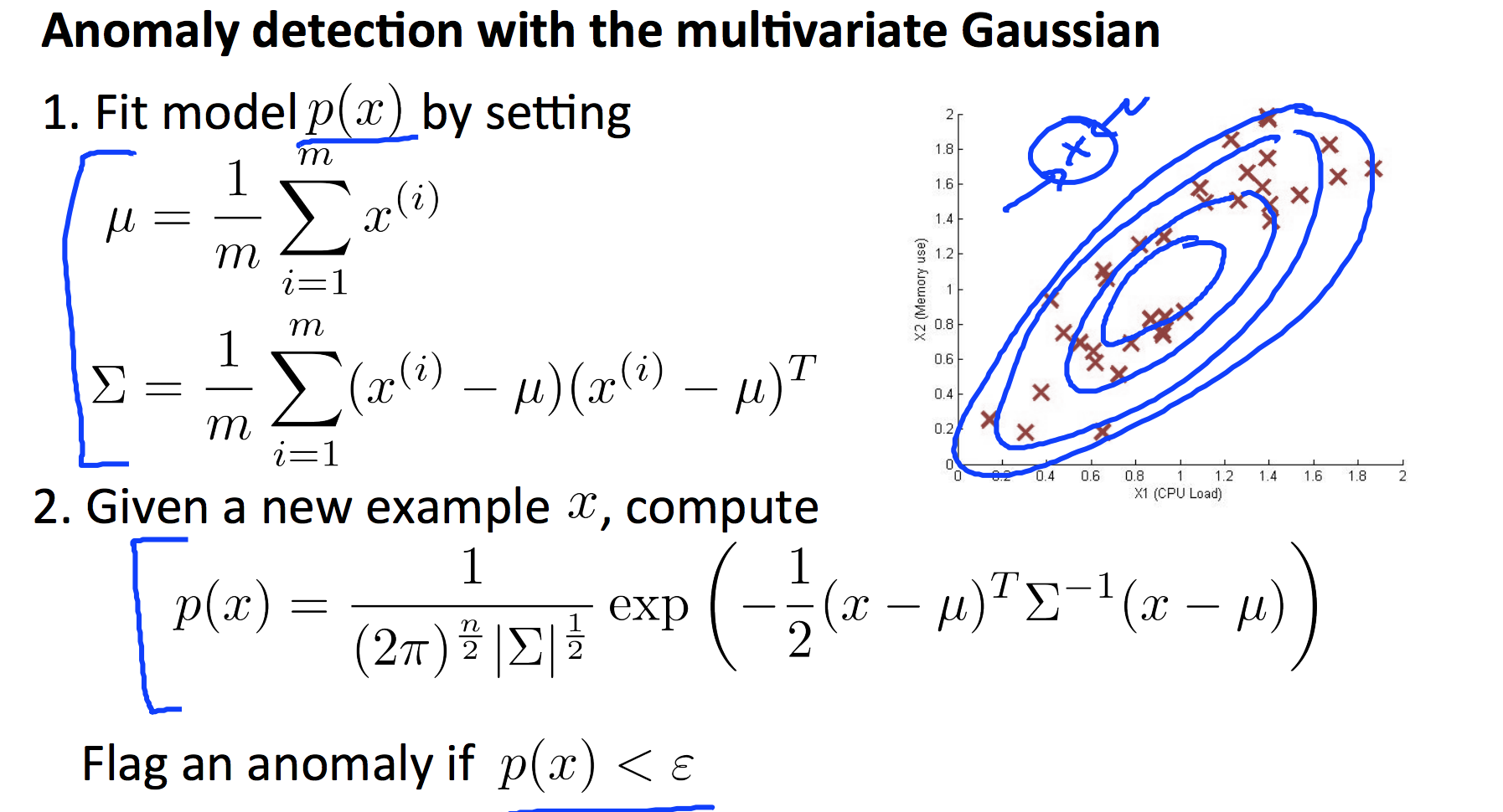
function [mu sigma2] = estimateGaussian(X)
%ESTIMATEGAUSSIAN This function estimates the parameters of a
%Gaussian distribution using the data in X
%   [mu sigma2] = estimateGaussian(X),
%   The input X is the dataset with each n-dimensional data point in one row
%   The output is an n-dimensional vector mu, the mean of the data set
%   and the variances sigma^2, an n x 1 vector
%

% Useful variables
[m, n] = size(X);
mu = zeros(n, 1);
sigma2 = zeros(n, 1);

% Instructions: Compute the mean of the data and the variances
%               In particular, mu(i) should contain the mean of
%               the data for the i-th feature and sigma2(i)
%               should contain variance of the i-th feature.
%
mu = mean(X)';
sigma2 = (var(X) * (m - 1) / m)';

end
function p = multivariateGaussian(X, mu, Sigma2)
%MULTIVARIATEGAUSSIAN Computes the probability density function of the
%multivariate gaussian distribution.
%    p = MULTIVARIATEGAUSSIAN(X, mu, Sigma2) Computes the probability
%    density function of the examples X under the multivariate gaussian
%    distribution with parameters mu and Sigma2. If Sigma2 is a matrix, it is
%    treated as the covariance matrix. If Sigma2 is a vector, it is treated
%    as the \sigma^2 values of the variances in each dimension (a diagonal
%    covariance matrix)
%

k = length(mu);

if (size(Sigma2, 2) == 1) || (size(Sigma2, 1) == 1)
    Sigma2 = diag(Sigma2);
end

X = bsxfun(@minus, X, mu(:)');
p = (2 * pi) ^ (- k / 2) * det(Sigma2) ^ (-0.5) * ...
    exp(-0.5 * sum(bsxfun(@times, X * pinv(Sigma2), X), 2));

end
9. Tips for Building a Learning System
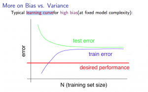
9.1 Bias and Variance
Learing Curve:
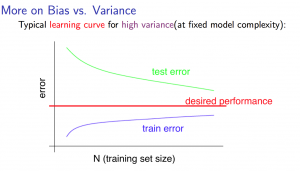
- Getting more training examples: Fixes high variance
- Trying smaller sets of features: Fixes high variance
- Adding features: Fixes high bias
- Adding polynomial features: Fixes high bias
- Decreasing λ: Fixes high bias
- Increasing λ: Fixes high variance.
9.2 About Dataset Separation
In order to choose the model and the regularization term λ, we need to:
- Create a list of lambdas (i.e. λ∈{0,0.01,0.02,0.04,0.08,0.16,0.32,0.64,1.28,2.56,5.12,10.24});
- Create a set of models with different degrees or any other variants.
- Iterate through the λs and for each λ go through all the models to learn some Θ.
- Compute the cross validation error using the learned Θ (computed with λ) on the JCV(Θ) without regularization or λ = 0.
- Select the best combo that produces the lowest error on the cross validation set.
- Using the best combo Θ and λ, apply it on Jtest(Θ) to see if it has a good generalization of the problem.
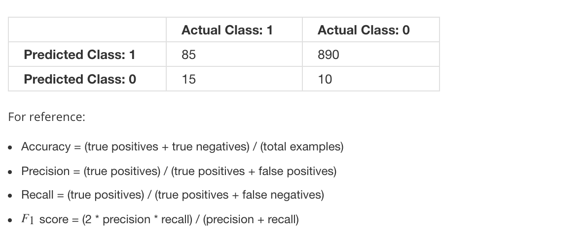
9.3 Metrics for skewed data
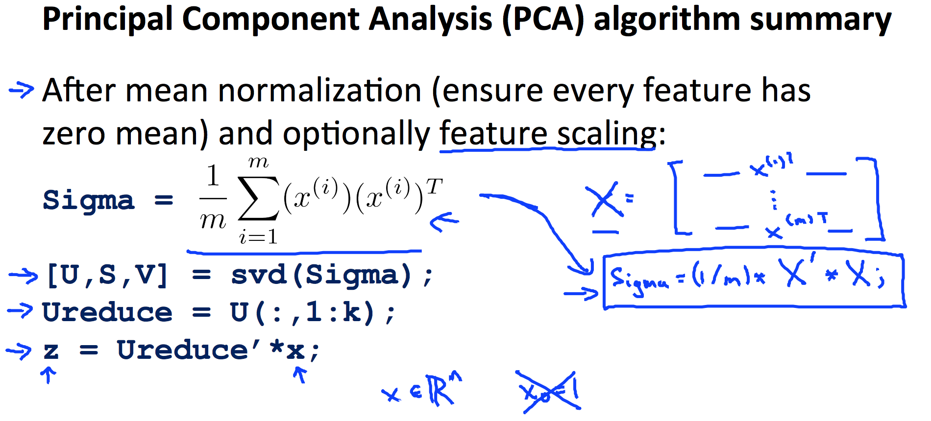
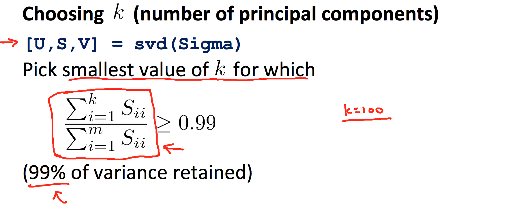
9.4 PCA
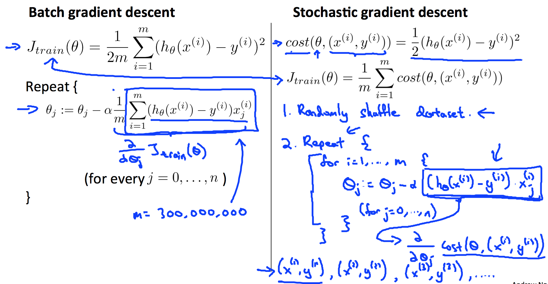
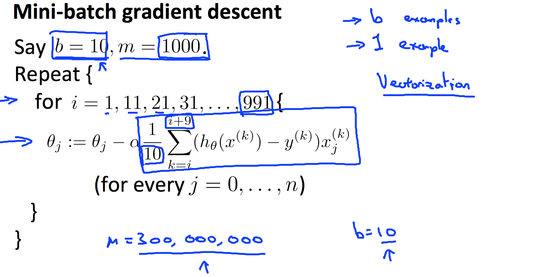
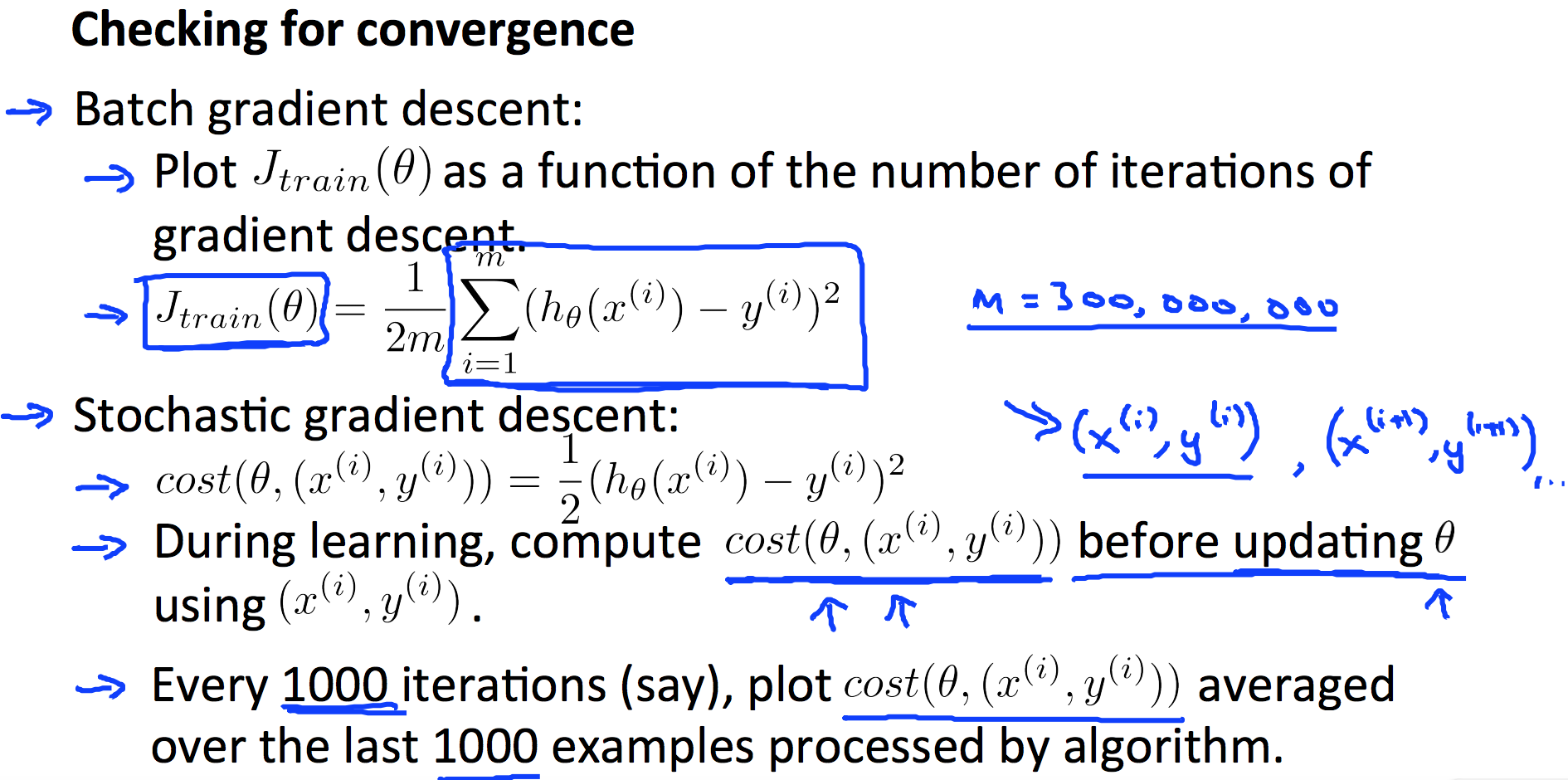
9.5 Stochastic and Mini-batch Gradient Descent
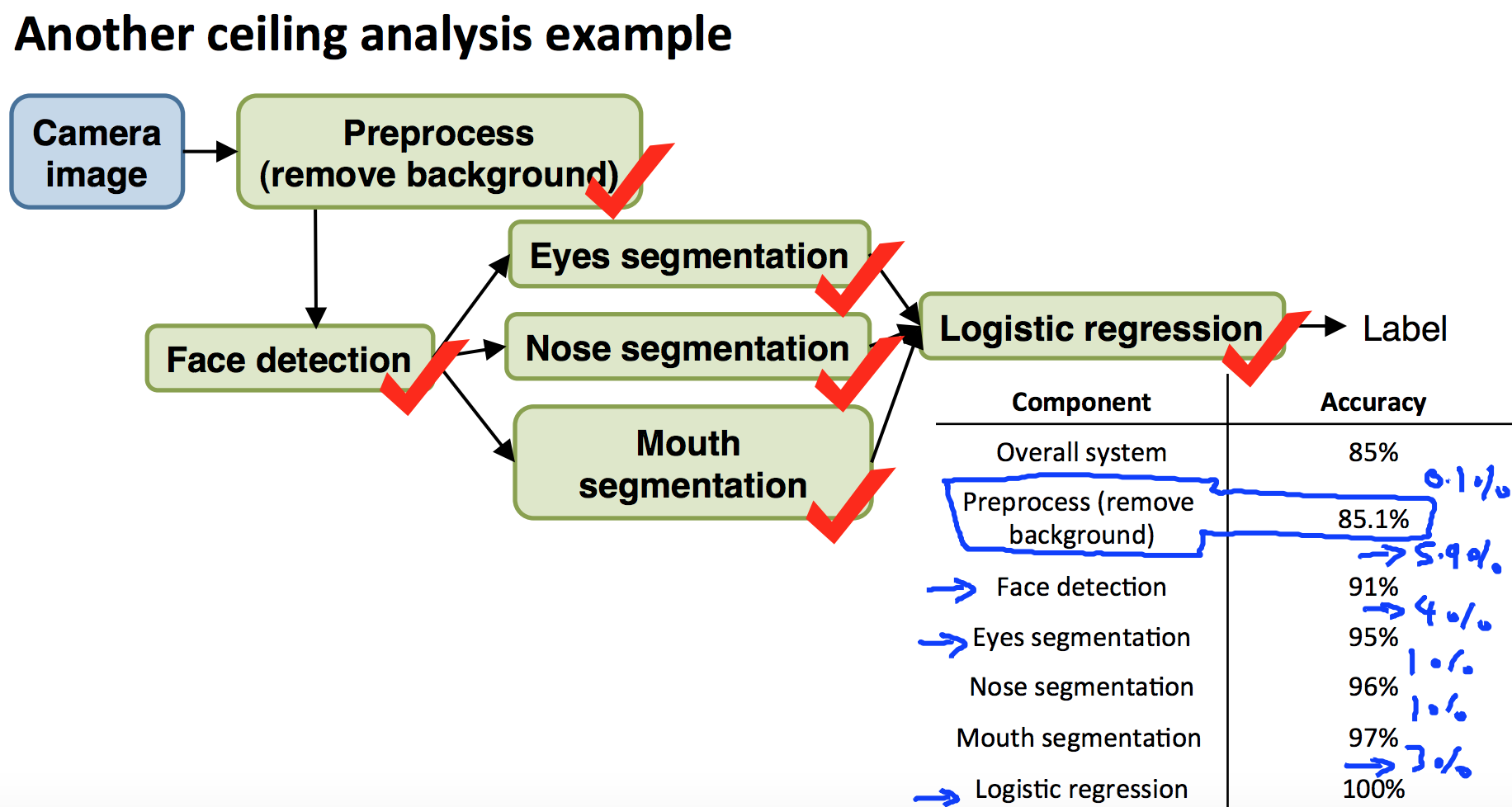
9.6 Ceiling Analysis